Demo 7
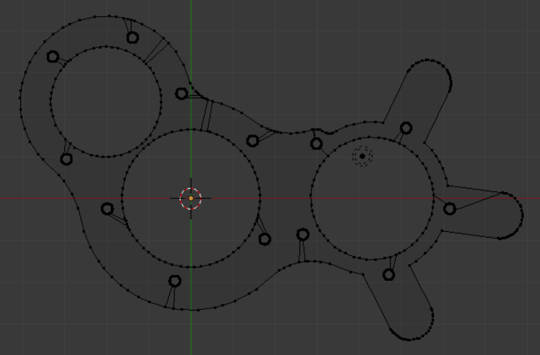
This object is a pump casing. It belongs to the INRIA model repository (see References). Hosted as a .stp file in the Elmer GUI samples folder, it is converted to an .obj by FreeCAD, and then imported by Blender. (The model can also be accessed in .stp and .stl format from the Aim Shape model repository.)
This object is a pump casing. It belongs to the INRIA model repository (see References). Hosted as a .stp file in the Elmer GUI samples folder, it is converted to an .obj by FreeCAD, and then imported by Blender. (The model can also be accessed in .stp and .stl format from the Aim Shape model repository.)
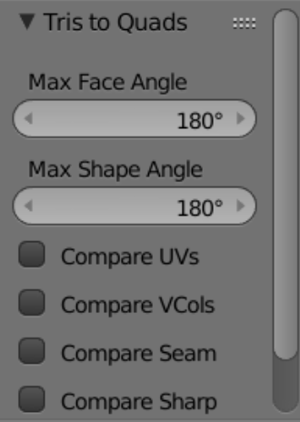
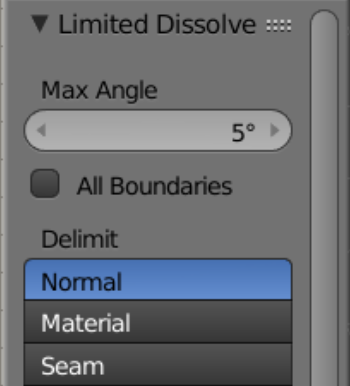
The commands ‘Mesh → Faces → Tris to quads’, and ‘Mesh → Cleanup → Limited Dissolve’ remove all traces of triangles and get the model ready to edit. The settings used in this case are pictured at right. The reason the flat surfaces of the mesh show very few edges is that they are just single big n-gons.
We hide everything except the top n-gon. The wireframe view in Blender’s Edit mode is the most convenient setting for doing the work. The tools to be employed are the knife tool, edge extrusion, and duplicate-and-move. When open gaps occur in the working plane of faces, and there is no n-gon surface to operate on, ordinary face making will take the place of the knife tool.
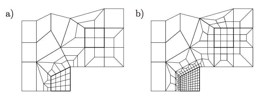
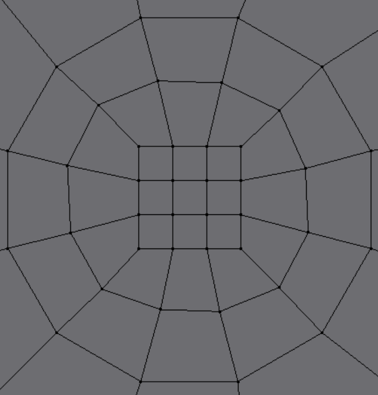
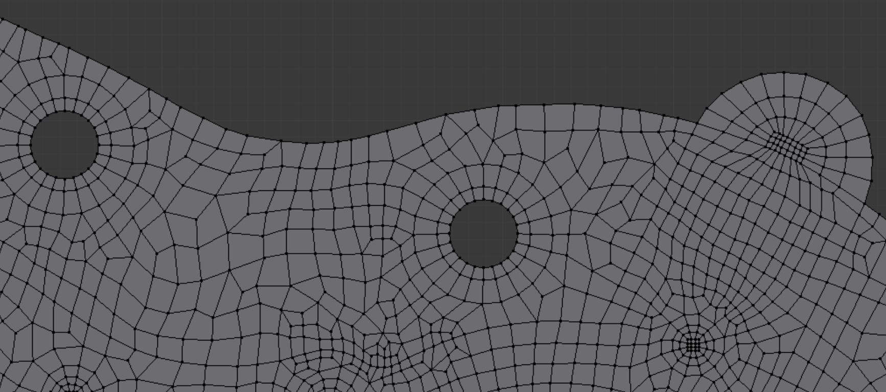
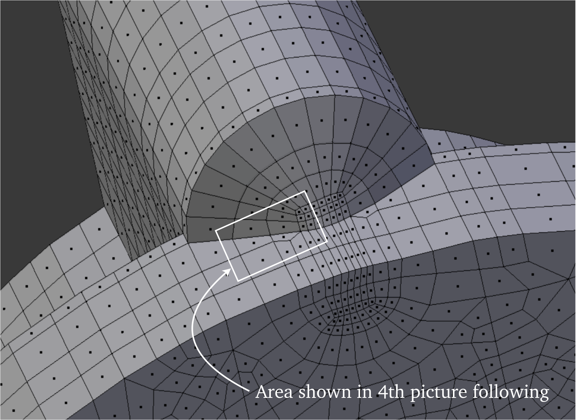
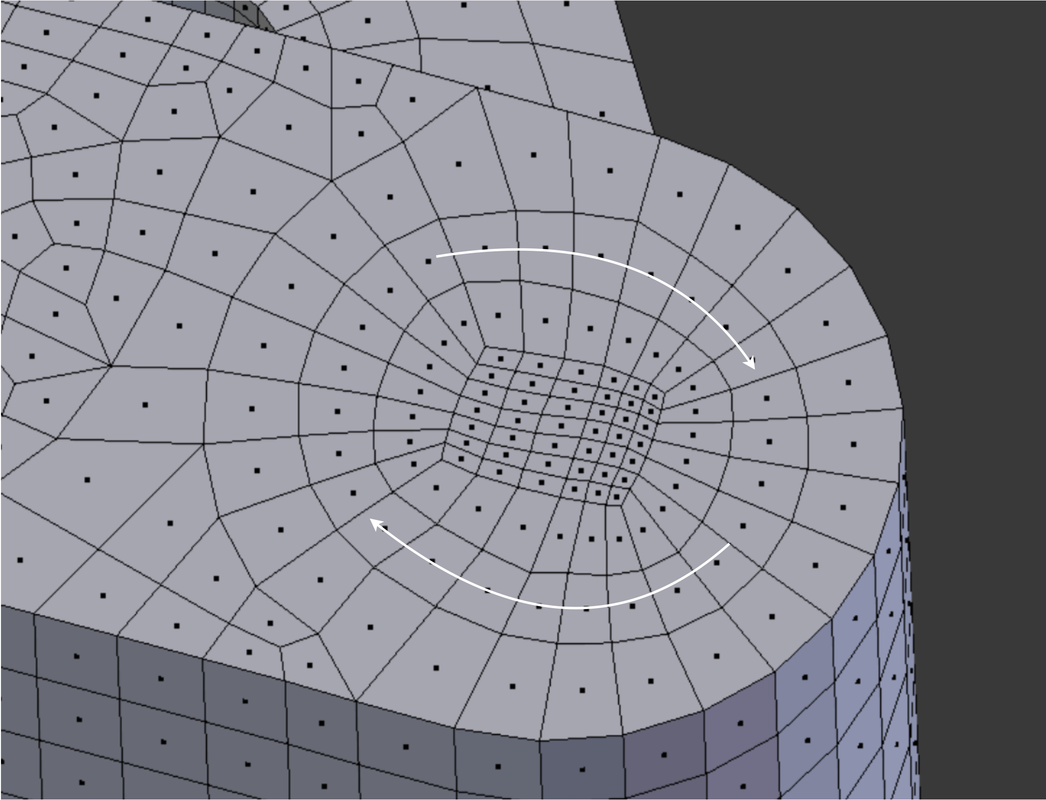
Two illustrations concerning transition zones, between different levels of detail, in quadrilateral mesh. For this and other useful illustrations, see Schneiders in References.
We elect to use 12-division hole bottoms and use Blenbridge to translate the appropriate pattern from Febio Preview, then import the resulting .ply into Blender.
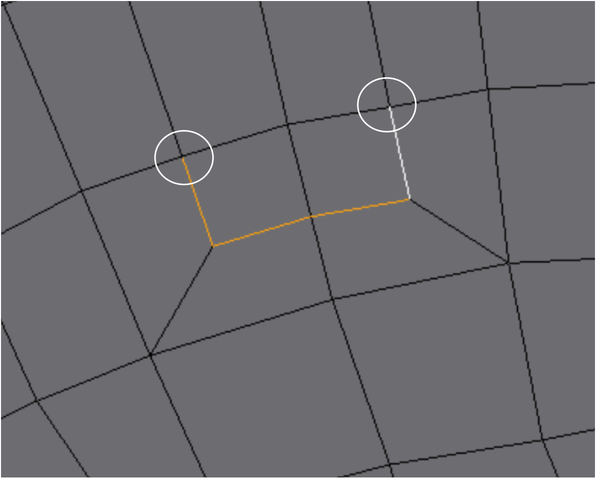
The tension of two loose-ended points (circled) can be balanced by creating a loop. However, if a match cannot be found for a surplus point, an exterior boundary point must be created or destroyed to maintain the balance.
Being careful to always remain in top view, we make the mesh. Because the view is perpendicular to a main axis, moving with ‘g’ (grab) does not disturb the flatness (much). This is the mainstay of smoothing operations on the mesh. When it is necessary to slide a vertex along an outside edge, we use Shift+‘v’ to do it.

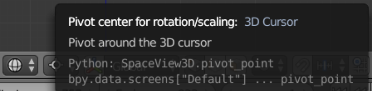
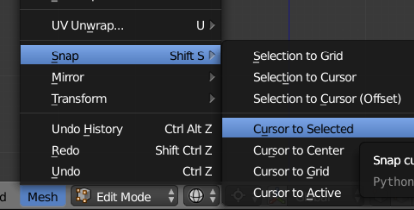
The zoomed mountainous region seen from a front view is only 0.007 Blender units high, but perfect flatness can be achieved easily. We first make sure the 3D cursor is the Pivot Center. Then we use Shift + ‘s’, followed by ‘u’, to snap the 3D cursor to a selected point with a z-value that we want all the points to have. Then we select all points and press ‘s’ (scale), then ‘z’ (axis), then 0, then Enter.
We stage the five working plates that will play parts in the vertical extrusion process. Each plate differs from the one above and below because of its characteristic features.
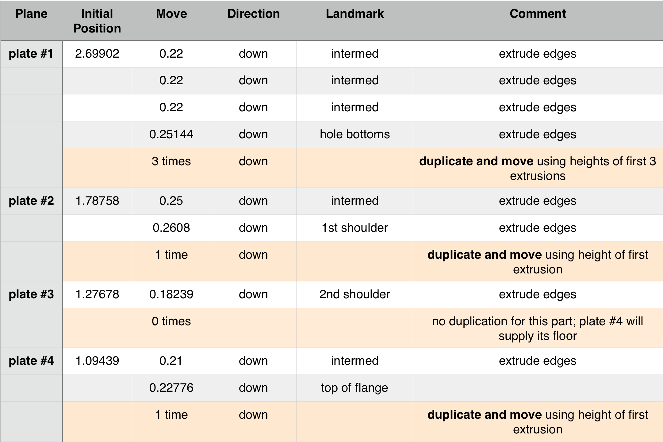
With a somewhat complicated generation course, we note down the various extrusion steps. Accuracy is a relative concept, but our goal here is to get the horizontal and vertical parts’s positions to match within the 0.0001 unit default separation of Blender’s ‘Remove Doubles’ function.
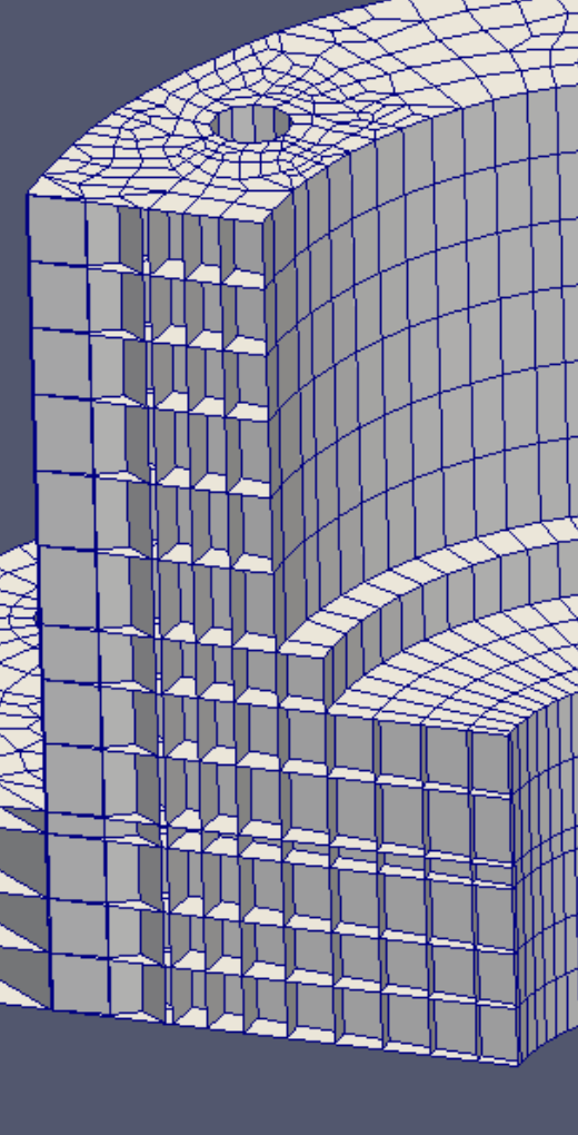
The construction process in progress. If necessary, we can switch out of wire frame for a moment to verify the 3D cursor location for a duplication, then go back into wireframe, press the ‘b’ key, and make the selection. In the above picture, the final as-yet unused plane is shown as the black line at the bottom. After the steps are completed, Blender reports the removal of 54,946 duplicate vertices.
One task which is needed after construction is to verify that the horizontal floors of the mesh all made it into the model. We can do this in Blender, or we can open the mesh in Paraview and apply a Clip filter to the .ply file to have a look inside.
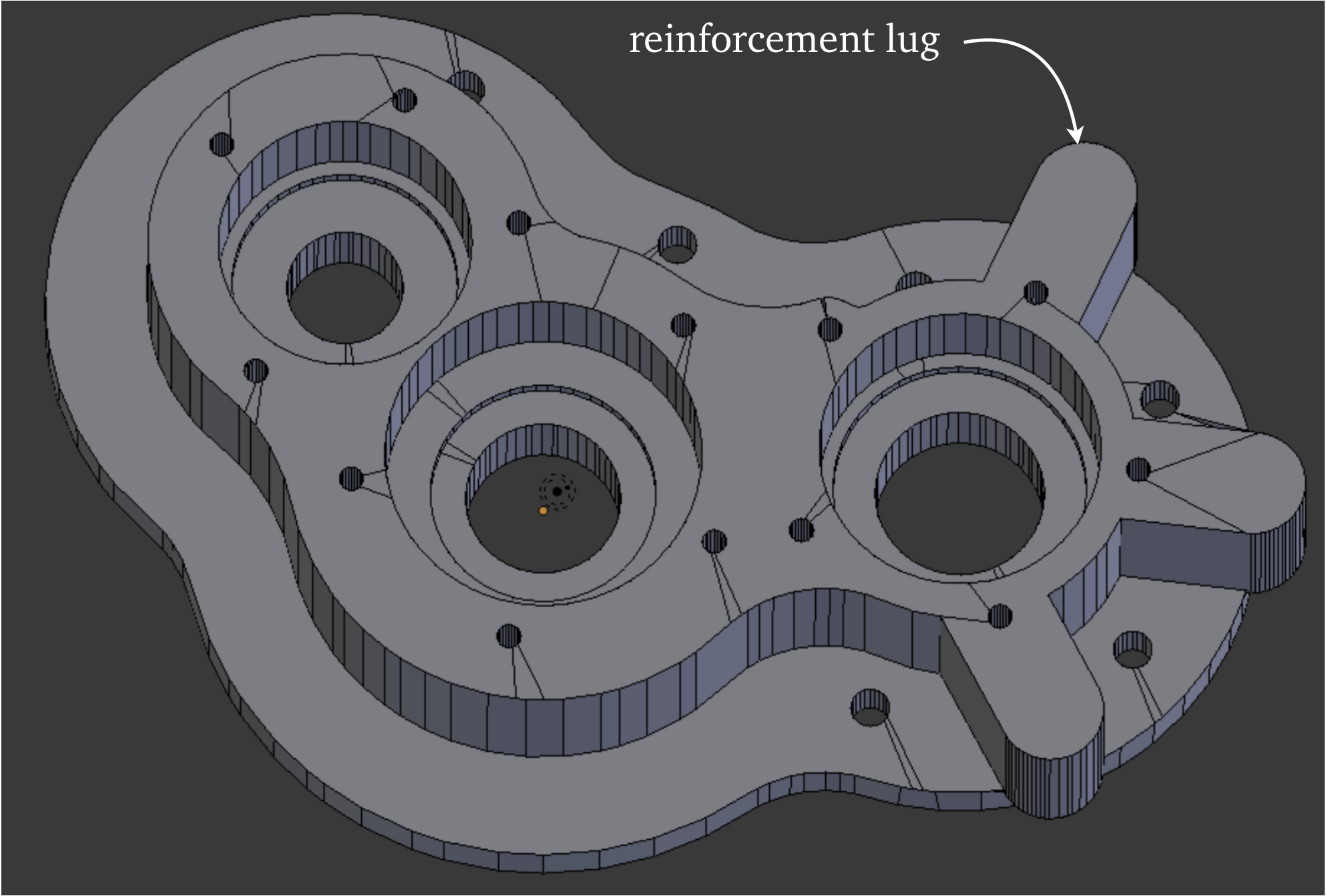
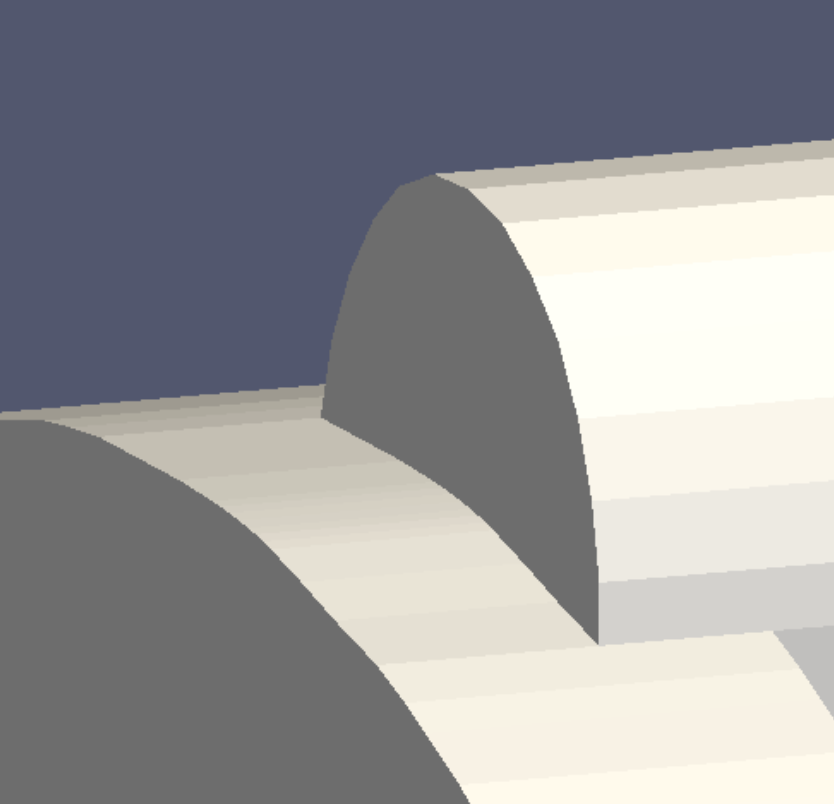
On a first attempt we choose to “de-feature” the conical treatment of the bottoms of the reinforcement lugs and make them flat, as shown below, due to their negative mesh quality impact. However, after consideration, the look of greater authenticity contained in the picture below right tempts us to look further into the problem.
On a first attempt we choose to “de-feature” the conical treatment of the bottoms of the reinforcement lugs and make them flat, as shown below, due to their negative mesh quality impact. However, after consideration, the look of greater authenticity contained in the picture below right tempts us to look further into the problem.
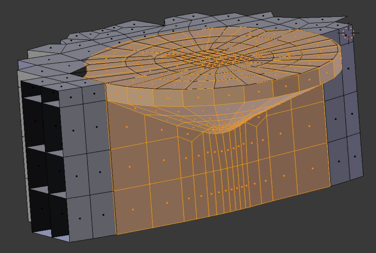
The original model contains the surfaces making up the cones. We desire these surfaces. We use the lug pattern incorporated in our mesh to knife project at full scale down through the original structure, then merge the original into ours, thus capturing the surface contours.
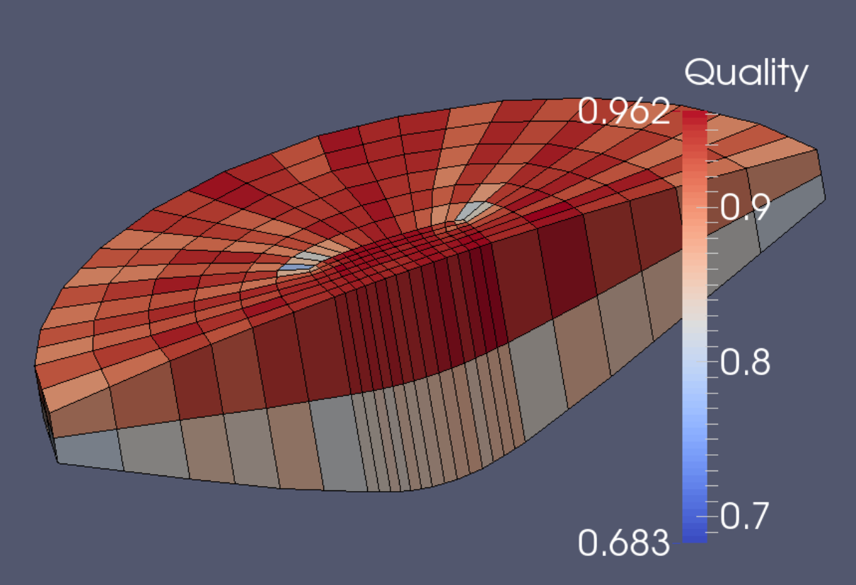
After the Scaled Jacobian quality turns out well, we are encouraged to seek a way to incorporate the cones into our mesh.
After the Scaled Jacobian quality turns out well, we are encouraged to seek a way to incorporate the cones into our mesh.
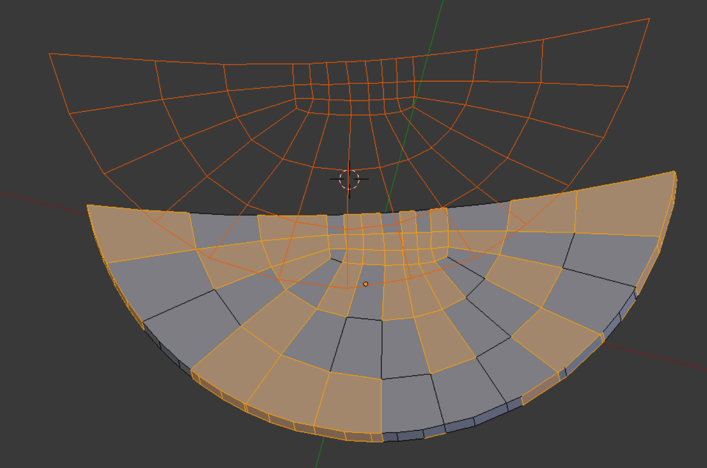
The key concept is reflection. Any nonconforming edge structure is given a reflection path, so that it does not carry back into the main mesh. This strategy prevents excessive proliferation of elements in the main structure.
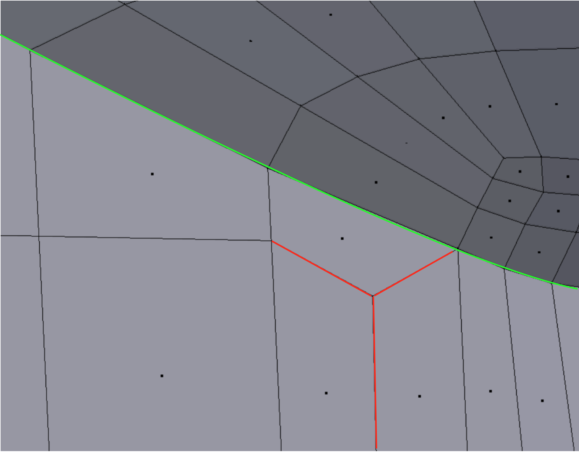
At the interface between cone and flange. The edges outlined in green are handled by conforming the existing edge network in way of the cone. The edges outlined in red are reflected.
We will see this approach again, in Demo 22.
After the fashioning of a successful cone subassembly for one reinforcement lug, the basic pattern is adapted and reused on the other two. Slight accommodations are necessary to suit individual sites.
The Verdict score for Diagonal measure is also seen to be acceptable.
The Diagonal score was facilitated by use of the method of Demo 6 of the documentation of the program Lifted (see References).
The Diagonal score was facilitated by use of the method of Demo 6 of the documentation of the program Lifted (see References).
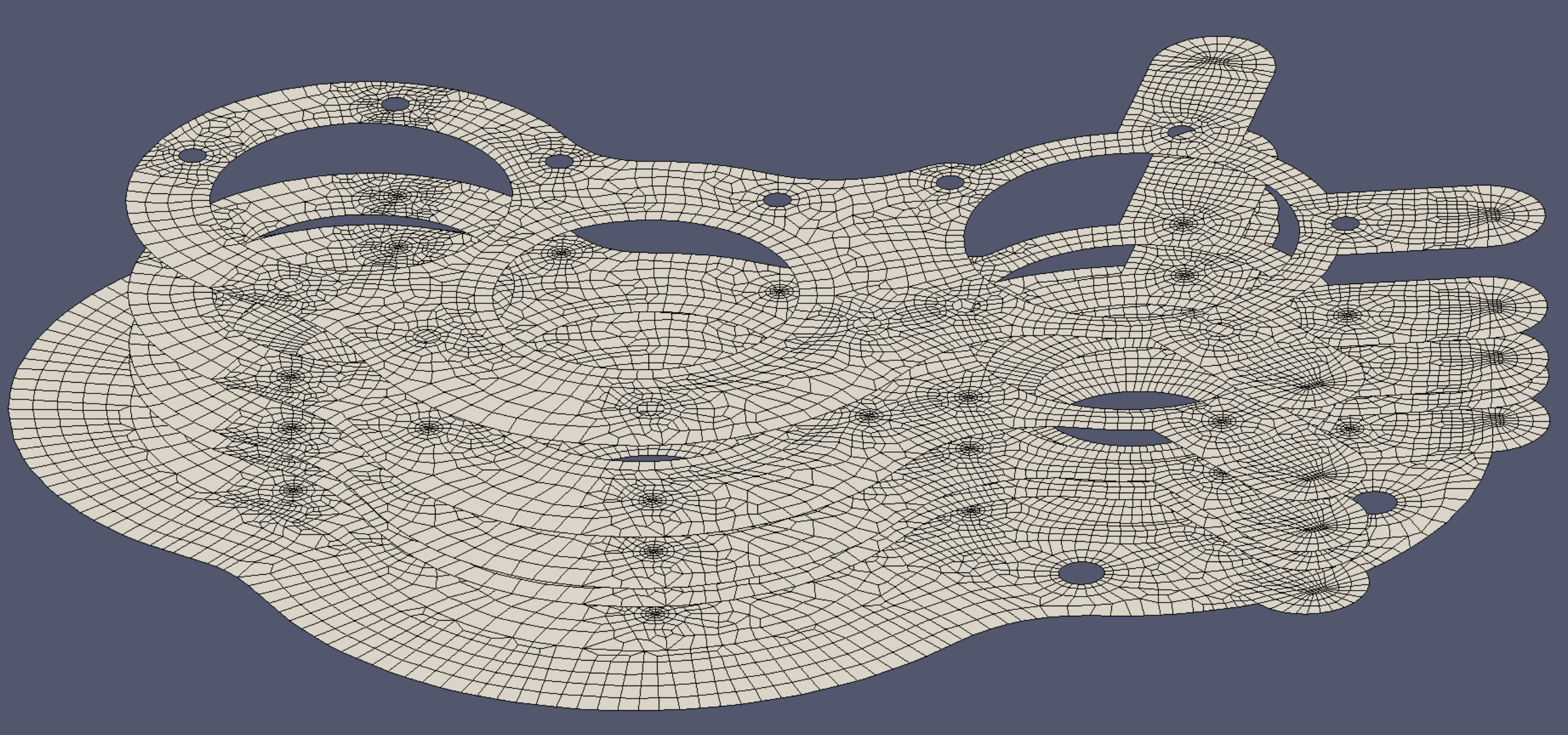
The final mesh is shown in Elmer GUI. With 16GB of ram, we could possibly carry out either a heat transfer calculation or tackle a structural mechanical problem, assuming we are using an iterative solver, the type which Elmer has.
For the final mesh, we allow Gmsh to refine and split it. This results in 404,480 elements and 444,215 nodes. For Blenbridge to convert the .ply file to .vtk format for this rather large model requires 44 minutes 44 seconds on a recent Macbook.
For the final mesh, we allow Gmsh to refine and split it. This results in 404,480 elements and 444,215 nodes. For Blenbridge to convert the .ply file to .vtk format for this rather large model requires 44 minutes 44 seconds on a recent Macbook.
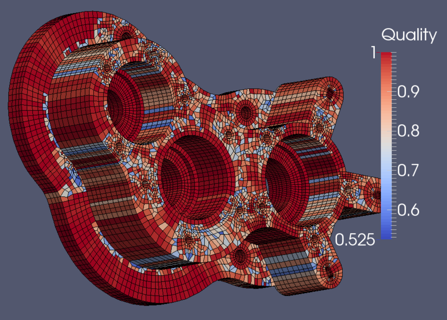
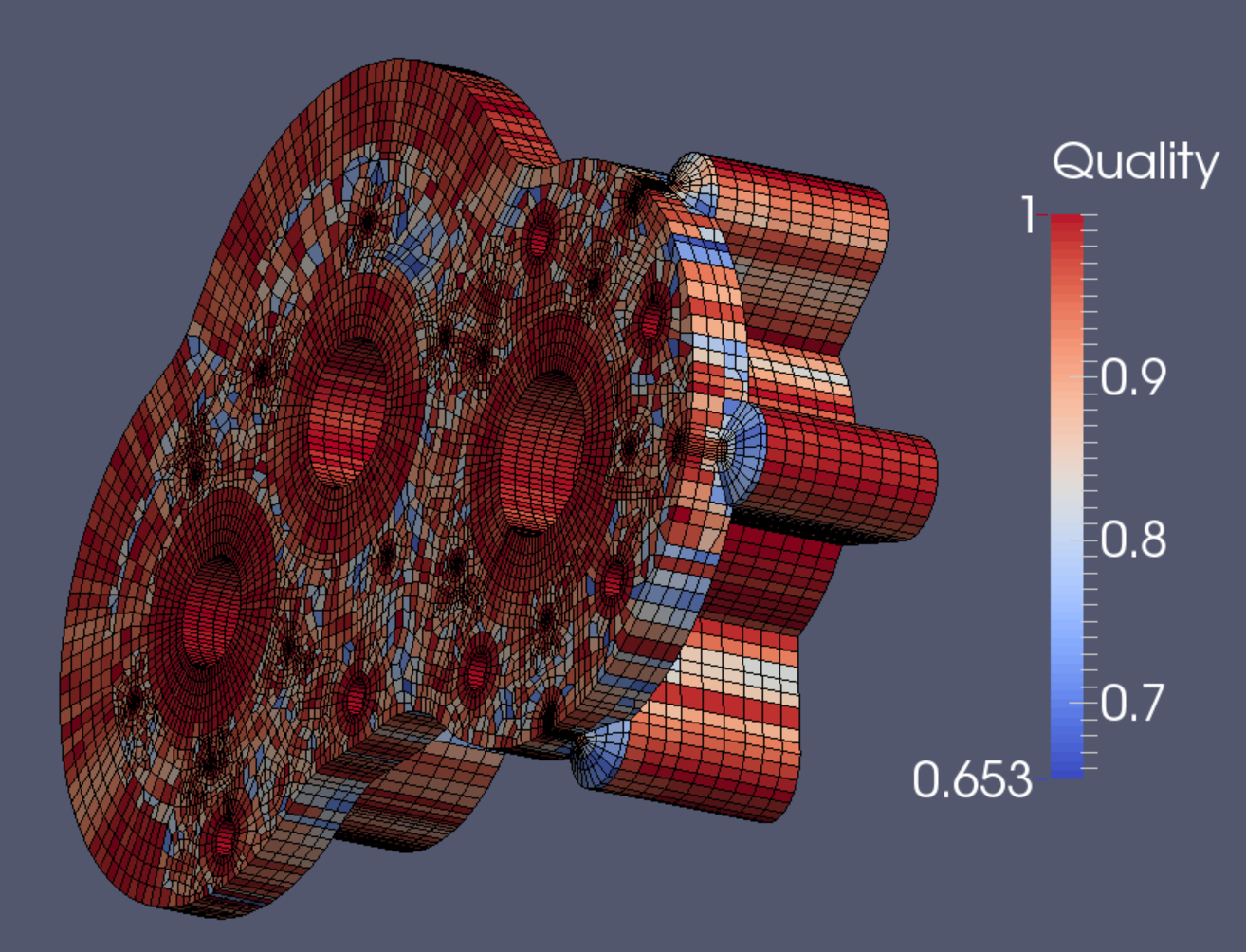
The final mesh quality check is favorable, showing a minimum Scaled Jacobian score of 0.525.
The mesh shown has 50,560 elements and 60,582 nodes.
The mesh shown has 50,560 elements and 60,582 nodes.